Acknowledgements
This work has been supported by the Swedish
Natural Science Research Council, which is gratefully acknowledged. I also
would like to thank my supervisor Prof. Stig Lundqvist for introducing me to
the field of dynamical systems, chaos and fractals. My other supervisors Prof.
Mats Jonson and Dr. Predrag Cvitanovic, is gratefully acknowledged for all
their advice and discussions that came up under this work. I also want to thank
Dr. Gunnar Nicklasson for introducing me to fractal aggregate and practical use
of fractals and Dr. Gunnar Russberg for his valuable comments on this
manuscript. Finally, I want to thank all my colleagues at Chalmers and NORDITA
in Copenhagen.
1. INTRODUCTION
One question one may ask about fractals is: Why do we need non-integer
dimensions? A short answer to the question is that for some strange objects it is
not possible to find a well-defined measure (other than zero) without introducing non-integer or fractal dimensions.
What this means will be explained later in the thesis.
A fractal object in three-dimensional space is
characterized by a large surface-to-volume ratio. For example, the need of a
rapid gas exchange explains the existence of the large surface-to-volume ratio
observed in a lung. The area of a human lung measured with the resolution 100
µm is as large as that of a tennis-court (has the size of 102 m2) while the volume enclosed by it is a few litres [1] (has the size of
10-3 m3). Another case where a large surface-to-volume
ratio is needed, is for the materials used for efficient catalysis. A
characteristic property of a fractal is that its measure depends on the resolution used in the measurement. Typically, the surface area of an object
converges very fast to a finite limiting value as the resolution is increased,
but for fractals the area diverges
The theory of fractals radically differs from
traditional Euclidean geometry, fractal geometry describes objects that are
self-similar, or scale invariant. This means that when some parts of such an object
is magnified, it is seen to bear an exact resemblance to the whole, the
likeness continuing with the parts of the parts and so on to infinity. The
self-similar structure is perhaps the main reason for the striking beauty of so
many fractals [2]. A set is strictly self-similar if it can be expressed as a
union of sets, each of which is a reduced copy of (is geometrically similar to)
the full set. However, not all fractal objects exhibit this precise form. In a
coastline, for instance, there is an irregular nesting of gulfs, bays,
harbours, and coves that are observed over a broad range of spatial scales. A
magnified view of one part of the coastline may not precisely reproduce the
full picture, but it will have the same qualitative appearance. A coastline
displays the kind of fractal behaviour that is called statistical
self-similarity. Fractals also must be devoid of translational symmetry--that
is, the smoothness associated with Euclidean lines, planes, and spheres.
Instead a rough, jagged quality is maintained at every scale at which an object
can be examined. The nature of fractals is reflected in the word itself, coined
by Benoit B. Mandelbrot, [3] derived from the Latin verb frangere, "to
break," and the related adjective fractus, "irregular and
fragmented." His book "The
Fractal Geometry of Nature (1982)" is the standard reference and
contains both the elementary concepts and an unusually broad range of new and
rather advanced ideas, such as multifractals, currently under active study.
The simplest fractal is the Cantor bar (named
after the 19th- century German mathematician Georg Cantor). It is constructed
by dividing a line in 3 intervals and removing the middle interval. The
procedure is repeated indefinitely, first on the 2 remaining intervals, then on
4 intervals produced by that operation, and so on, until the object has an
infinitely large number of intervals each of which is infinitely small.
Fractals are not relegated exclusively to the
realm of mathematics. If the definition is broadened a bit, such objects can be
found virtually everywhere in the natural world. The difference is that
"natural" fractals are randomly, statistically, or stochastically
rather than exactly scale symmetric. The rough shape revealed on one length
scale bears only an approximate resemblance to that on another, but the length
scale being used is not apparent just by looking at the shape. Moreover, there
are both upper and lower limits to the range in size over which the fractals in
nature are indeed fractal. Above and below that range, the shapes are either
rough (but not self-similar) or smooth--in other words, conventionally
Euclidean.
Whether natural or mathematical, all fractals
have particular fractal dimensions. These are not the familiar Euclidean
dimensions given by integers--1, 2, or 3--but a different kind of quantity. Usually
noninteger, a fractal dimension indicates the extent to which the fractal
object fills the Euclidean dimension in which it is embedded. A natural fractal
of fractal dimension 2.8, for example, would be a sponge-like shape nearly
3-dimensional in appearance. A natural fractal of fractal dimension 2.2 would
be a much smoother object that just misses being flat.
The roots of fractal geometry can be traced to
the late 19th century, when mathematicians started to challenge Euclid's
principles. Fractional dimensions were not discussed until 1919, however, when
the German mathematician Felix Hausdorff[4] put forward the idea in connection
with the small-scale structure of mathematical shapes. As completed by the Russian mathematician A.
S. Besicovitch, Hausdorff's dimensionality was a forerunner of fractal
dimensionality. Other mathematicians of the time, however, considered such
strange shapes as "pathologies" that had no significance.
This attitude persisted until the mid-20th
century and the work of Mandelbrot. His 1961 study of similarities in large-
and small-scale fluctuations of the stock market was followed by work on
phenomena involving nonstandard scaling, including the turbulent motion of
fluids and the distribution of galaxies in the universe. A 1967 paper on the
length of the English coast showed that irregular shorelines are fractals whose
lengths increase with increasing degree of measurable detail. By 1975,
Mandelbrot had developed a theory of fractals, and publications by him and
others made fractal geometry accessible to a wider audience. The subject began
to gain importance in the sciences. As mentioned, fractal geometry appears in
many fields of science, in the study of landscapes (e.g., coast lines,
mountains, rivers and sediments), in the study of plants, metals and composite
materials, in crystals, aggregates, flows, galaxy formations, populations and in economical systems etc.
The dimensions and scaling indices also characterise universality classes of
systems. They are equal for systems of a given class, since they describe the
same scaling properties.
Mandelbrot later also investigated another
fractal terrain, that of shapes distorted in some way from one length to
another. These fractals are now called nonlinear, since the relationships
between their parts is subject to change. They retain some degree of
self-similarity, but it is a local rather than global characteristic in them.
The general definition of the word fractal may thus need further refinement, to
indicate more precisely which shapes should be included and which excluded by
the term.
The most intriguing of the nonlinear fractals
thus far has been the mathematical set named after Mandelbrot by the American
mathematicians John Hubbard and Adrien Douady. The more the set is magnified,
the more its unpredictability increases, until unpredictability comes to
dominate the bud-like shape that is the set's major element of stability. The
set has become the source of stunning colour computer graphics images. It is
also important in mathematics because of its centrality to dynamical system
theory. An entire Mandelbrot set is actually a catalogue of dynamical
mathematical objects--that is, objects generated through an iterative process
called Julia sets. These derive from the work done by a French mathematician,
Gaston Julia, on the iteration of nonlinear transformations in a complex plane.
Scientists have begun to investigate the
fractal character of a wide range of phenomena[5], [6]. Researchers are
interested in doing so for the practical reason that behaviour on a fractal
shape may differ markedly from that on a Euclidean shape. Physics is by far the
discipline most affected by fractal geometry. In condensed-matter, or
solid-state physics, for example, the so-called "percolation cluster"
model used to describe critical phenomena involved in phase transitions and in
mixtures of atoms with opposing properties is clearly fractal. This has
implications, as well, for a host of attributes, including electrical conductivity.
The percolation cluster model may also apply to the atomic structure of
glasses, gels, and other amorphous materials, and their fractal nature may give
them unique heat-transport properties that could be exploited technologically.
Mathematical physics, for its part, has a
particular interest in nonlinear fractals. When dynamical systems--those that
change their behaviour over time--become chaotic, or totally unpredictable,
physicists describe the route they take with such fractals. Called strange attractors,
these objects are not real physical entities but abstractions that exist in
"phase space," an expanse with as many dimensions as physicists need
to describe dynamical physical behaviour. One point in phase space represents a
single measurement of the state of a dynamical system as it evolves over time.
When all such points are connected, they form a trajectory that lies on the
surface of a strange attractor. Most physicists who study chaos do so with
carefully controlled laboratory setups of turbulent fluid flow. Individual
strange attractors have been identified for different kinds of turbulent fluid
flow, suggesting the existence of numerous routes to chaos [7], [8], [9].
Although not concerned with fractals to the
same extent as physics, other sciences have discovered them. In biology, the
anomalous thermal relaxation rate of iron-containing proteins has been
explained as resulting from the fractal shape of the linear polymer chain that
comprises all proteins. The
distribution pattern of atoms on the protein surface, a different aspect of
protein structure, also appears to be fractal. Many more fractals have been
detected in geology, including both random exterior surfaces--ragged mountains
and valleys--and interior fractal surfaces in the brittle crust, such as
California's famous San Andreas fault. Earthquake processes for small
tremors--those of magnitude 6 or less--appear to be fractal in time as well as
space, since these quakes occur in self-similar clusters rather than at regular
intervals. Meteorology provides a different kind of space-time fractal: the
contour of the area over which tropical rain falls is self-similar, and the
amount of rain that falls varies in a self-similar fashion over time. Finally,
on the interface of science and art, computer-graphics specialists, using a
recursive splitting technique, have produced striking new fractal images of
great statistical complexity. Landscapes made this way have been used as
backgrounds in many motion pictures; trees and other branching structures have
been used in still lifes and animations.
Another major area of condensed-matter physics
to invoke the concept of self-similarity is that of kinetic growth, in which
particles are gradually added to a structure in such a way that once they stick,
they neither come off nor rearrange themselves. In the case of the simplest model of kinetic growth, the most
important physical phenomenon to which it applies appears to be the fingering
of a less-viscous fluid (water) through a more viscous fluid (oil) lodged in a
porous substance (limestone and other kinds of rock). A more complex model
explains the growth of colloidal agglomerates.
FRACTAL DIMENSION
Fractal dimension can be defined in many ways, but before giving a definition I
would like to discuss how to measure the size of general (fractal) objects. Since we want to measure objects
with varying degree of resolution, we cover them by boxes, squares or
line-segments and count how many are needed for a complete covering. In the
following we will call squares and line-segments boxes (in two and one
dimension respectively) as well. The objects are covered/enclosed in d-dimensional boxes of
size l,
where d
is the topological dimension of the set. The topological
dimension is always an integer. The fractals we will discuss may be considered
to be sets of points in coordinate space or in phase-space. They may be single
isolated points like galaxies in the Universe or molecules combined to
complicated patterns like aggregates. The set of points that make up a line in Euclidean space has the
topological dimension d = 1, and the fractal dimension D = 1. The set of points
that form a sheet has d = 2 , D = 2 and a ball d = 3 and D = 3.
2.1: Measuring general sets
To illustrate the general method of measuring,
consider a smooth curve in Euclidean space, see Fig. 1.
Figure 1. The total measure (length, area and volume) of the curve is
found by counting the number of boxes needed for the covering, multiplied with
the box-size (l, l2, l3) in the limit
l ® 0.
The measure (here the length) of the curve is found by counting the number of
equally sized line-segments of length l, N(l), needed to cover the curve. The total length is
then given by
![]() (1)
(1)
since the number of segments needed to cover the curve is inversely
proportional to the segment size, i.e., N(l) µ l-1 = L0l-1. In the limit l ® 0 the
measure asymptotically equals the length of the curve and is independent of l. If we instead
measure the area of the curve we replace the line-segments by a grid of
squares. The total area of the curve is then given by
![]() (2)
(2)
Similarly the volume of the curve is zero. We
observe that the only interesting measure of a curve is the length, i.e., the
only meaningful dimension of a curve is d = 1.
If we instead consider a set of points defining
a smooth surface in Euclidean space, we cover the set with squares of size l2 and counts the number
of squares needed to cover the set, see Fig.
2.
Figure 2. The total measure (length, area and volume) of a surface is
found by counting the number of boxes needed for the covering, multiplied with
the box-size (l, l2, l3) as l ® 0.
The measure of the area is then given by
![]() (3)
(3)
where N(l) µ l-2 = A0l-2. Similarly we can
define a "length" and a "volume" of the surface by
![]() (4)
(4)
and
![]() (5)
(5)
As we can see, the only interesting measure of a surface is the area. In other words; the only interesting dimension
for the study of an ordinary smooth surface in Euclidean space is d = 2. However, one may
easily define sets of points that are curves, which twist so badly that their
length is infinite (see the triadic Koch curve below, in the limit n ® ∞). Some curves, so called Peano curves even fill the plane. Before
discussing such strange sets we have to generalize the measure of size for a
given set.
In general, the d-dimensional measure is defined as
![]() (6)
(6)
where N(l) is the number of boxes of size l needed to cover the
curve and d
the topological dimension of the set. As l ® 0, three things may
happen. 1) If d > D, the measure diverges; 2) if d < D, the measure becomes zero. Only when 3) d = D the measure may approach a finite, nonzero
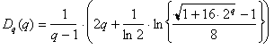
value. Thus, by requiring Md to be constant (not zero), we define the value
of the critical dimension D which we will refer to as the fractal
dimension. In the literature there exist alternative definitions of fractal
dimension [3-6]. The important property in the calculation of fractal
dimensions is how the number of boxes needed to cover the set scales with the
box-size. This means that if N(l) µ l-D in the limit l ® 0, only d = D gives a finite
measure since
![]() (7)
(7)
We may therefore determine the fractal dimension of an object from the slope of ln N(l) plotted as a
function of ln l (see
e.g. Fig. 5). An object will be
called fractal if its observed measure depends on the resolution (box-size)
over several orders of magnitude, and follows a “power law” behaviour with a
nontrivial exponent. This dependence can be observed over an infinite range of
the resolution in the case of fractals generated by mathematical constructions.
Such fractals have no smallest and no largest scale. In contrast, fractals used
to model growth processes like aggregation of magnetic particles (see paper III)
have a smallest scale due to a finite particle size. However, such fractals can
be made from a mathematical construction. This can be made by halting the
iteration at a finite level as the snowflake fractal in paper II. In real
physical systems, there also exists a lower cut-off for the box-size since the
fractal structure is replaced by different patterns when approaching the
microscopic scales. Therefore a straight line in the plot of ln N(l) vs. ln l can be observed
only in some range of l. This range must extend over several decades
in order to imply the existence of a fractal structure.
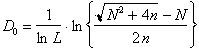
2.2: A
one-scaled Cantor set (part
1)
A very simple method to construct fractal sets with a fractal dimension in the range 0 < D < 1 is
shown in Fig. 3.
Figure
3. The first three steps in the
construction of a one-scaled Cantor set. At each stage of construction the central third of each segment is
removed from the set. For the resulting fractal D = 0.631...
One starts out with a unit interval [0,1] and
replaces it by N smaller intervals. In the example a unit
interval is replaced by two new intervals of length 1/3. By repeating the procedure on each of the
remaining intervals ad infinitum one gets a set of remaining points called a
one-scaled Cantor set. The simple construction of the set makes it easy to
calculate the fractal dimension, since we know the number of intervals (boxes) on any level of
construction. Let us use a grid obtained by dividing the unit interval into 3n equal intervals (n is a fixed integer).
As follows from the construction, the number of such pieces (of size 3-n) needed to cover the
Cantor set is 2n.
We then have l = 3-n and N(l) = 2n which gives
![]() (8)
(8)
This measure diverges or approaches zero, unless we choose
d = D = ln 2/ln 3 = 0.6309... From the generalised measure we can then
define the fractal dimension as
![]() (9)
(9)
Since the Cantor set is given by a mathematical
construction (a recursive rule) the scaling behaviour exist over an infinite range of
resolution. A fractal as the Cantor set is called a deterministic fractal since it can be constructed by a deterministic rule. The Cantor set is
also a self-similar object. Such objects can be
divided into N identical parts, each being a rescaled
version, by a factor r, of the complete set. Let N1(l) denote the number of boxes on a grid of size l << L (L is the size of the
fractal) needed to cover one such part. The number of boxes needed to cover the
complete fractal is then
![]() (10)
(10)
Due to the self similarity, N1(l) equals the number of boxes needed to cover the
complete set with boxes of size l/r, i.e.,
![]() (11)
(11)
The fractal dimension is then given by
![]() (12)
(12)
which is an exact result for one-scaled fractals [3].
2.3: Coast
lines and the triadic Koch curve
A
common example of fractal objects is coastlines. The length of a coastline
depends critically on the length of the yardstick used to measure the distance
between points along the coast. Smaller yardstick gives a larger measure of the
coast.
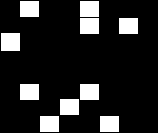
Figure
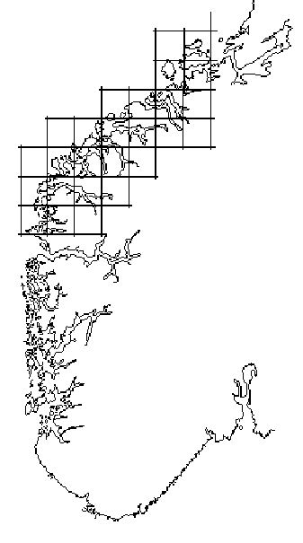
4. The coast of the southern part of Norway. The outline was traced from an
atlas and digitized at about 1800 x 1200 pixels [12]. The shown grids has a size l ~ 50 km.
Fig. 5 shows how the measured length increases as the
yardstick length, l, is reduced. This log-log plot shows that the measured coastline shows no sign to
reaching a fixed value as l is reduced. In fact, the measured length is
nicely approximated by the formula
![]() . (13)
. (13)
If we suppose the coast to have a well defined
length LN we would
expect it to be LN, at least for small enough l, and the exponent
should be equal to one. However, for the coastline of Norway, see Fig. 4 the value of D is found to be 1.52 [12].
In Fig. 6
we show a reproduction of the data collected by Richardson (from Mandelbrot's
(1982) book [3]) showing the apparent length of various coastlines and
boundaries. They all fall on straight lines in the log-log plot except for the circle for which the measure converge
to a finite value.
Figure
5. The measured length of the coast of Norway as function of the yardstick l.
The straight line in this log-log plot corresponds to the relation L(l) = a . l 1 - D, with D » 1.52.
The slope of the lines in the plot is 1 - D, where D is the fractal
dimension of the coastline. As model for such a coastline we will study a
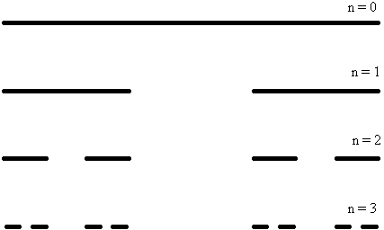
simple set called the triadic Koch curve, (see Fig. 7). The set is
constructed from a unit interval, which we call the 0-th generation of the Koch curve.
By replacing this interval by the polygon
marked n = 1 we get the first generation of the set. If we then continue and replace
each of the four segments with a new polygon and so on, we get in the limit n ® ∞ a fractal set. Since the set is
generated by the polygon marked n = 1 this polygon is called the generator of the Koch
curve.
Figure
6. The length of coastlines as a function of the yardstick length (Mandelbrot,
1982).
The Koch-curve has in the limit n ® ∞ an infinite length, an area A = 0, and therefore
not a well-defined measure in an integer dimension. At a given level n the curve consists of 4n segments, each of
length 3-n. We then find the
fractal dimension of the Koch curve to be
![]() (14)
(14)
The topological dimension of the set must be
equal to one since we can stretch the curve to a straight line after each step
in the construction. We then conclude that the Koch curve is a fractal set with dimension
D = ln 4/ln 3.
Figure
7. The construction of the triadic Koch curve. By replacing each line segment
with a resized copy of the part marked n = 1 we construct a fractal with D = ln 4/ln3.
2.4: Some
simple fractals in d = 2
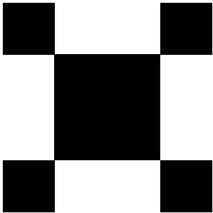
In two dimensions it is easy to construct
fractal sets by instead of using an interval, using a square and removing parts
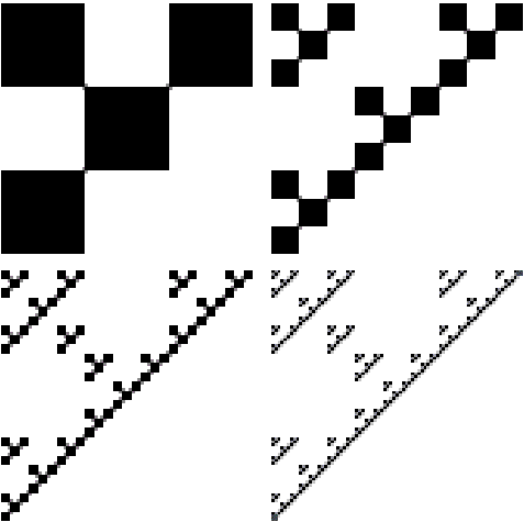
of it recursively. First we prove that we can construct a one-dimensional set
by partitioning a unit square into nine new squares and removing six of them as
shown in Fig. 8. Repeating the
procedure with the three remaining squares ad infinitum, we end up with a
straight line. The size of the squares at level n is (1/3)n and the number of squares of that size needed
to cover the set is 3n. We get D = 1 just as we can expect. Since the topological
dimension d = 1, the remaining set is not a fractal.
Figure 8. The construction of a
"fractal" set with D = 1.
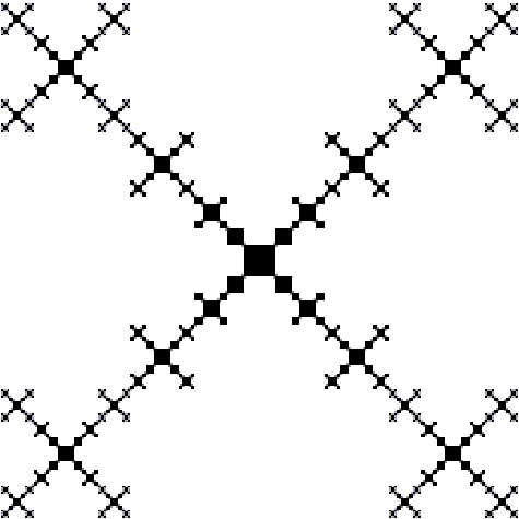
If we instead construct a snowflake by dividing
a square into nine parts and remove four of them (see Fig. 9) we get in the limit l ® 0 (
<=> n
® ∞) 5n squares of size (1/3)n and then D = (ln 5)/(ln
3).
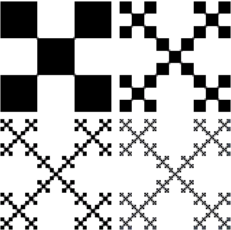
Figure 9. A one-scaled snowflake
fractal.
We observe that if we remove six squares we get
D = 1.
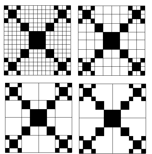
It is possible to generate different fractal sets with the same fractal
dimension. This is illustrated in Fig. 10
and Fig. 11 where we have divided two
squares in nine pieces and removed five of them recursively. Both have the
fractal dimension D = ln 4/ln 5.
Figure
10. A fractal measure of dimension D =
ln 4/ln 5. Compare this fractal with Fig 11. which has the same fractal
dimension.
Figure 11. A second fractal measure of dimension D = ln
4/ln 5. Compare this set with the set in Fig 10.
3. MULTIFRACTALS
We have so far only studied objects that are fully characterized by a
single value D, the Hausdorff
dimension, henceforth denoted by D0. Fractals found in
nature however, most often need for their characterisation a whole spectrum of
dimensions called generalized dimensions
Dq. The Hausdorff dimension is only one dimension
in this continuous spectrum. Such fractals are called multifractals. The
essential difference between the construction of multifractals and (one-scaled)
fractals is that the initial set is divided into N not identically sized parts. Each sub-set is a
reduced version of the original object by some factor. The procedure is
repeated self-similarly ad infinitum.
A starting point in the study of multifractal
objects is the construction of a partition function G [13]. The set is covered with a grid of boxes
numbered i = 1, 2, ..., N of (for simplicity of equal) size l. N = N(l) is the total
number of boxes of size l needed
to cover the set. The probability to find some part of the fractal in box i, pi, is then equal to the
number of points in the box (= ni) divided by the total
number of points in the complete set, i.e., the total normalized mass, M = ∑ni. The partition
function is then given by
![]() (15)
(15)
where t is called the mass exponent ,, q the moment
order , and li is the
length of the i´th box. In Eq. (15)
we assume that all lengths li have the same size l.
Depending on t
and q
three things may happen in the calculation of G.
If for fixed q, t is
greater than some t(q) the partition sum
diverges to infinity. On the other hand, if t
is less than t(q) the sum converges to zero. Only if t is exactly equal to t(q) the sum approaches a finite value different
from zero
 . (16)
Compare this with the discussion of general measure in section 2.1, Eq. (7). Thus,
by requiring G = constant (not zero) we define the
relationship between t and q. If we normalize the
probabilities pi i.e.,
∑ pi = 1, give G = 1.
The function t(q), sometimes called the free energy, is then given by
![]() (17)
(17)
We then define the generalized dimensions Dq [14 -
17] as
![]() (18)
(18)
i.e.,
![]() (19)
(19)
If we put q = 0 we get the original expression for the
Hausdorff dimension
![]() (20)
(20)
For a uniform fractal, with all pi equal (not a multifractal), one obtains a
general dimension Dq that does not vary with q. For a non-uniform
fractal, (multifractal) however, the variation of Dq with q quantifies the non-uniformity. For instance
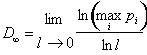 (21)
(21)
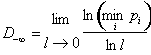 . (22)
For a multifractal the Dqs are positive numbers which decrease
monotonically with q and for simple (one-scaled) fractals all the Dqs coincide.
Now, assume the following scaling relation for
the probability of the i'th box in the limit l ® 0
![]() (23)
(23)
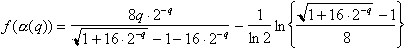
where ai is position independent. This relation defines
the scaling index ai also called the crowding index
or the Lipschitz-Hölder exponent.
Since a controls the singularity of the density, it may
also be called the exponent of the
singularity. The same scaling relation can be
found in many boxes (for small l), and all boxes with the same scaling index
are said to be a sub-fractal with a point wise dimension ai. This sub-fractal is said to have a dimension f(ai). In other words, the function f(a) can be interpreted as the
Hausdorff dimension of the set of points with the
same point wise dimension a. For a simple fractal like the one scaled Cantor set the function f(a) is only defined in a single
point (a, f) = (D0, D0) (see example below).
Such a fractal is not a multifractal. In contrast, for multifractals a is no
longer unique but may take on values in a finite range [amin, amax],
while f(a) turns out to be, in general, a
single humped function with D0 as its maximum. To find the relationship
between f(a) and t(q) we re-express the partition sum as an
integral in a. We then get
![]() (24)
(24)
where ![]() is the number of
times a' assumes a value in the interval [a',a'+da']. In the limit l ® 0, the dominant contribution to the
integral is received when the exponent
is the number of
times a' assumes a value in the interval [a',a'+da']. In the limit l ® 0, the dominant contribution to the
integral is received when the exponent ![]() is close to its
minimum value, so we perform a saddle-point approximation
is close to its
minimum value, so we perform a saddle-point approximation
![]() (25)
(25)
This leads to the following Legendre
transformation [13], which is used to determine the f(a)
spectrum
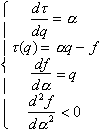 (26
a-d)
(26
a-d)
From these equations we note that the function f(a) is a convex function with a
slope q
in each dense point. As q ® ∞
the largest pi (i.e., the most concentrated part of the
multifractal) dominate the partition function. This corresponds to the point where the f(a) curve vanishes with infinite
slope, which is at the leftmost part for the minimum a. As q ®
-∞ the smallest pi dominate (i.e., the least concentrated part)
and the corresponding a-value, the rightmost part
of the f(a) curve vanishes with negative
infinite slope. By increasing (decreasing) the exponent q, boxes with higher
(lower) probabilities, i.e., fractal regions with denser (more ramified)
occupation, are selected. We then see that the contribution of the partition
function of different powers of the box probabilities is dominated by a
different fractal subset. For q = 1 the generalized dimension is of special importance. From
the relation ![]() and its derivative taken at q = 1 we find D1 = a1 = f1 where
and its derivative taken at q = 1 we find D1 = a1 = f1 where
![]() (27)
(27)
The quantity D1 thus measures how the information scales with ln l. Therefore D1 is called the information dimension [18, 19]. The function S(l) is called the entropy of the fractal. Moreover, this concept has been used to give a precise
definition of a multifractal [19]. A distribution is said to be a multifractal
measure if its Hausdorff dimension D0 exceeds its information dimension D1. In a similar way one
can show that the dimension D2 measure the correlation between the
probabilities pi and is therefore called the correlation dimension of the set.
3.1: The
box-counting method
In box-counting we cover the fractal with boxes
of different sizes and count the number of particles in each box. For
simplicity, we use boxes of equal size, (1/2)m, m = 1, 2, ..., mp where ![]() is the size of the
smallest particle in the fractal. We never use boxes of size smaller than the
smallest particles, since this gives no new information. The probability pi to find a particle in
a box i
is then given by the number of particles in the box, ni, divided by the total
number of particles in the fractal N. With known probabilities and box-size, we can
construct the partition function, G(t,q) Eq. (15) and calculate the fractal dimensions Dq, Eq. (19). From Eqs.
(17) and (26 a) we get the scaling exponent
is the size of the
smallest particle in the fractal. We never use boxes of size smaller than the
smallest particles, since this gives no new information. The probability pi to find a particle in
a box i
is then given by the number of particles in the box, ni, divided by the total
number of particles in the fractal N. With known probabilities and box-size, we can
construct the partition function, G(t,q) Eq. (15) and calculate the fractal dimensions Dq, Eq. (19). From Eqs.
(17) and (26 a) we get the scaling exponent
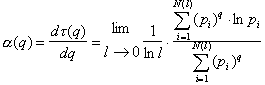 (28)
(28)
which is used with Eq. (18) to find the f(a)-spectrum:
![]() . (29)
. (29)
In section 3.6 we continue the discussion about box-counting by studying
the snowflake fractal used in paper I and paper II. This box-counting algorithm
is called fixed-size box-counting. Another possibility is to use an algorithm
called the fixed-mass box-counting, which consists in evaluation of the
required box size to accumulate an amount of measure µ Î [µmin, µmax]. It is specially appropriate to the evaluation of multifractal indices
with q £ 0.
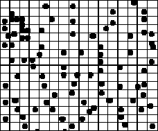
A pattern Fig. 12(a) is discretized and stored in a matrix Fig. 12(b) of pixels
with unit area (lmin2 = 1, in pixel units).
The measure, µ is also discretized by assigning a real number pi to each nonempty box.
The measure contained in each box, centred at random in a real domain with real
size l,
takes into account the fraction of pixels that are embedded in it. For the box-counting
fixed-size algorithm the procedure consists in covering the pattern with grids,
randomly located, of several lengths l in order to have several values pi(l). For the box-counting fixed-mass algorithm the
procedure consists in evaluating several lengths li(p), of boxes randomly
located in the aggregate which contain a measure p. When using box-counting on the snowflake multifractal below we will use the fixed-size algorithm for all values
of q,
and without moving the grid. One problem with fixed-size box-counting is that,
since the boxes will not necessarily be centred on particles on the fractal,
some of the boxes will contain spuriously small measure (probability), thus
creating problems for negative q-values. This is a difficult problem when
box-counting is used to calculate the f(a) spectrum for a general fractal, such as an
aggregate.
(a) (b)
(c)
Figure 12. In (a) we see a
pattern with 89
particles in a grid of size 1/16. The
mass of a particle is then normalized to be 1/89. Most
of the boxes are empty but some contains one two or at most three particles.
Figure (b) shows the boxes containing mass. The probability pi in each box then vary between ≈ 1/89 to ≈ 3/89. At
next box-level (c) the most of the boxes contains mass. For an accurate
calculation the need of moving the original grid becomes of importance.
3.2: The
one-scaled Cantor set (part
2)
To illustrate the difference between a simple
fractal and a multifractal we begin by studying the one-scaled Cantor set. First we construct the partition-function G. Since the Cantor set at level n consist of 2n intervals of size 3-n the partition
function is given by
![]() (30)
(30)
To find the function t(q) we take the
logarithm of Eq. (30). We then get
![]() (31)
(31)
i.e.,
![]() (32)
(32)
The generalized dimensions Dq is then given by Eq. (19), i.e.,
![]() (33)
(33)
which is the same as the Hausdorff dimension D0 found in section 2.2. From Eqs (26a) and (32)
we get the scaling exponent a
![]() (34)
(34)
and finally from Eq. (26b) we get
![]() (35)
(35)
i.e., a = f(a) = Dq = D0 as we
expected for a one-scaled fractal.
3.3: The
two-scaled Cantor set
To get a non-trivial f(a) spectrum we will next consider the
simplest multifractal we can imagine, namely a two-scaled Cantor set as shown in Fig. 13. The
set is constructed by dividing the unit interval in two pieces of different
lengths, L = 1/2 and l = 1/4, respectively, and repeating the dividings
self-similarly ad infinitum. The measures (probabilities) of the intervals are
then P = 2/3 and p = 1/3 (if pi ~ li).
Figure
13. A Cantor set construction with two rescalings L = 1/2 and l = 1/4 with
probabilities P = 2/3 and p = 1/3. The division of the set continues
self-similarly ad infinitum.
The partition function G at the first level of construction, i.e., for n = 1 is given by
![]() (36)
(36)
Similarly, at the next level G will be
![]() (37)
(37)
and at a general level n, the partition function G, is given by
![]() (38)
(38)
The simple partition function is due to the recursive
constructions of the Cantor set. Since we have a normalized measure (P + p = 1) the
partition function Gn = 1 " n, i.e., G is
independent of n. Such a partition function is called a generator. To find the f(a) spectrum for this set we first have to
find the function t(q) and then use the Legendre transformation Eqs. (26a) and (26b). The
function t(q) can be found by solving the equation
![]() (39)
(39)
with Newton-iterations. If the probabilities (P and p) are proportional to
the respective length (L and l) i.e., P = L/(L + l) and p = l/(L + l), equation can be reexpressed as a second order
polynomal and then we can find an analytical expression of t(q) (see below). If we assume P > p the first term
of Eq. (39) dominates for large positive q-values. We then have
![]() (40)
(40)
and
![]() (41)
(41)
similarly, for large negative q:s, the second term of Eq. (39) dominates,
i.e.,
![]() (42)
(42)
and f(a) = 0. The generalized dimensions in these limits are given by
![]() (43)
(43)
and
![]() (44)
(44)
From the analysis above and the fact t(1) = 0 (see Eq. (17)), we can now plot the shape of t(q), Dq and f(a) (see paper I). In general those curves look like the curves in Fig.
(14) - (16).
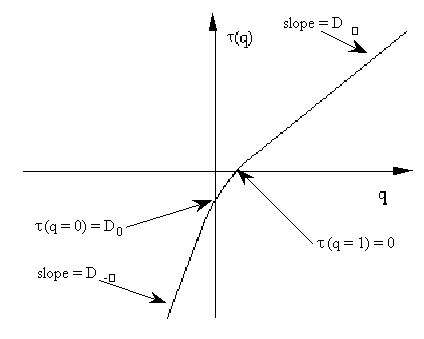
Figure
14 The general shape of the function t(q).
For large negative q-values t(q) = q . D-∞ - f-∞ and for large positive q:s t(q) = q . D∞ - f∞.
Remark D-∞
= amin and D∞
= amax.
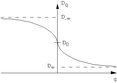
Figure
15. The general shape of the function Dq, D0 = fmax.
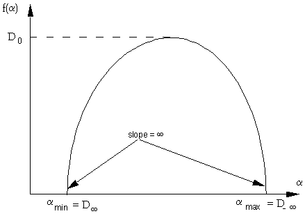
Figure
16. The general shape of the function f(a).
In the first step of the Cantor set construction, the set consists
of tree parts, a large interval L, a hole h and a small interval l. We denote this set
by (L, h, l)
or just (L, l). The next generation can be constructed by a multiplication:
(L + l)·(L + l) = L2 + Ll + lL + l2. (45)
This set is denoted by (L2, 2Ll, l2). The length of each
interval is given since L = 1/2 and l = 1/4. The next generation is given by (L3, 3L2l, 3Ll2, l3) and so on. We now observe that the Cantor set at level n only consists of n + 1 different scales.
We also observe that the number of boxes of size 2-n (= the size of the largest interval) is a
Fibonacci number and we can calculate the
Hausdorff dimension by studying two nearby levels m - 1 and m. The Fibonacci numbers are defined by
![]() (46)
(46)
The Fibonacci numbers are closely related to the golden mean
![]() . (47)
. (47)
We have in particular
![]() (48)
(48)
Since the partition functions Gm and Gm-1 have to be equal we can then use ![]() as
as ![]() to find D0. This gives
to find D0. This gives
![]() (49)
(49)
and
![]() (50)
(50)
which is the same result as was found in paper I.
3.4: Exactly
solvable recursive sets
There exists a set of recursive
multifractal objects which are exactly solvable. We will in this section study
such sets with two rescalings. The partition function for a general two-scaled
recursive set is given by
![]() (51)
(51)
where N is the number of segments of length L with probability P and n the number of
segments of length l with probability p on the first level of construction. This
equation is exactly solvable if l = L2 (< 1) and if the
probabilities P and p are proportional to their respective length
and normalized i.e., NP + np = 1. Then G = 1 and
![]() (52)
(52)
and
![]() (53)
(53)
where d is the topological dimension of the set. From
the expression (51) for the partition function one gets
![]() (54)
(54)
This equation can be reexpressed as a second
order polynomal If we set
x = Ldq - t, we get
![]() . (55)
. (55)
Equation (55) has a positive and a negative
root. We ignore the negative one since a negative length is irrelevant. The
positive root is
![]() (56)
(56)
Finally, we take the logarithm of Eq. (56). We then get the expression
for the function t(q).
 (57)
(57)
The generalized dimensions Dq are given by Eq. (18). Specially for the
Hausdorff dimension we get
 (58)
(58)
We also get the limits of Dq as
![]() (59)
(59)
and
![]() (60)
(60)
From the Legendre transformation (Eq. (26)) we
also have the f(a)-spectrum
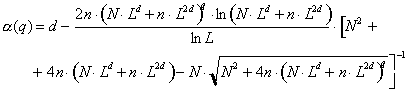 (61)
(61)
and
![]() (62)
(62)
If we apply Eqs. (47) - (62) on the two-scaled Cantor set where l = 1/2,
N = n = 1 and d = 1 we find
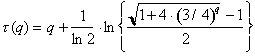 (63)
(63)
The Hausdorff dimension is then given by
![]() (64)
(64)
and the limits of the generalized
dimension by
![]() (65)
(65)
and
![]() (66)
(66)
Finally, the f(a) spectrum is given by
![]() (67)
(67)
and
![]()
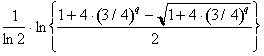 (68)
(68)
The generalized dimensions Dq and the f(a) spectrum for this Cantor set is shown in paper I.
A general recursive fractal set with a finite number, N of rescalings
![]() (69)
(69)
can be solved by Newton iterations. For each value of q we then solve Eq.
(69) to find the function t(q).
3.5: The
snowflake fractal
Another solvable multifractal is shown in Fig.
17 a-b. We call this multifractal a two-scaled snowflake fractal since it
reminds of a snowflake. This fractal is investigated in paper (II) and can be
used in the study of fractal aggregates.
Figure
17 a. The first level of construction of a two-scaled snowflake fractal
Figure
17 b The fourth level of construction of a two-scaled snowflake fractal
3.6:
Box-counting on the snowflake fractal
In this section the snowflake multifractal will be analysed in more detail.
From this example we learn a lot about box-counting. In paper II we show that it is possible to find analytic expressions
for the box-counting solution on any level of construction n, and for any level of
grids m,
i.e., box-sizes l = 2-m. Fig. 17a
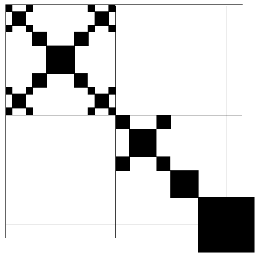
shows the multifractal at the first level of construction. If we call the "particle size" the size of the
smallest square in the set, the number of particles will increase as 8n. The fractals in Fig.
17a then consists of 8 particles of size 1/4 (a) and 82 = 64 particles of size (1/4)2 = 1/16 (b) respectively.
The snowflake fractal is covered with boxes of
size (1/2)m, m = 1, 2, ..., mn where ![]() is the size of the
smallest square in the fractal. The largest square (the one in the centre) has
the size Ln = (1/2)n. We then calculate the probability pi i.e., the measure of the fractal in each box
i.
is the size of the
smallest square in the fractal. The largest square (the one in the centre) has
the size Ln = (1/2)n. We then calculate the probability pi i.e., the measure of the fractal in each box
i.
First we have to find a recursive rule to
construct the snowflake fractal at any level. In paper II we defined the
operator ![]() operating on a square
x by
operating on a square
x by
![]() . (70)
. (70)
If we let this operator act on a unit square, i.e., x º 1 we get 4l + L, where l is a new square of size 1/4 and L a new square if size 1/2. By repeated operation with ![]() on the new set (4l + L) we construct
any level of the fractal. On the fourth level (Fig. 17b) we have
on the new set (4l + L) we construct
any level of the fractal. On the fourth level (Fig. 17b) we have
256 squares of size 1/256: 256 l4
256 squares of size 1/128: 64 l3L, 64 lLl2, 64 Ll3 and 64 L2lL
96 squares of size 1/64: 16 l2L2, 16 lLlL, 16 Ll2L, 16 lL2l,
16
LlLl and 16 L2l2
16 squares of size 1/32: 4 lL3, 4 LlL2, 4 L2lL and 4 L3l, and
1 square of size 1/16: L4.
To calculate the fractal dimensions Dq and the f(a) spectrum we need to find the function t(q)
![]() (71)
(71)
for all n
and m,
where the coefficients ![]() are the number of
boxes with the same probability
are the number of
boxes with the same probability ![]() .
.
To find the coefficients we have to study the
snowflake for some levels and the possible box coverings. In Fig. 18 we show
the snowflake on level n = 2 and box levels m = 4, 3, 2 and 1. On this level the smallest particle have the
length (1/4)2 = 1/16. In the finest box resolution m = 4 we have 64 boxes all with the
same probability p = 1/64. The function(q) is then given by
![]()
which gives
![]() ,
,
![]()
and
![]()
The values of the dimensions above are the first approximation of the exact values which are given in the
limit n
® ¥ and m ® ¥. Due
to the small box-size we only get one value of the probability and then only one value of the fractal dimensions, Dq, a and f(a) independent of the
momentum q.
If we increase the box size a factor 1/2 we find the same result for the dimensions
since we then get 256 filled boxes of size 1/32 with probability 1/256. This shows that
the smallest box-size of interest is the same as the smallest particle.
Figure
18. This is the fractal at level n = 2
covered by boxes of level m = 4, 3, 2 and 1, i.e., the particle sizes is l = (1/4)2 = 1/16 and
the box sizes are (1/2)4
= 1/16, (1/2)3
= 1/8, (1/2)2
= 1/4 and (1/2)1 = 1/2 respectively.
If we decrease the box size to level, m = 3 we have 16 boxes with probability 2/64 and 8 boxes with probability 4/64 = 1/16. The function
t(q) then becomes
![]()
which gives a continuous function of
generalized dimensions with
![]()
and the limits
![]()
![]()
when q ® ± ¥ . The f(a)-spectrum in the same limits are given by
![]()
![]()
and
![]()
The next two levels (m = 2 and m = 1) gives the same results as level 2 and 1 for the snowflake at
level n = 3 below.
Let us study one more level of the snowflake
fractal, level n = 3. In Fig. 19 we show the upper left part of the
snowflake with box level m = 6. On this level the snowflake consists of 512 particles of size 1/64. The function t(q) is
then given by
![]() .
.
This gives the generalized dimensions
![]() ,
,
Figure 19. This is the upper left part of
the snowflake fractal at level
n = 3, covered by boxes of level m = 6, i.e., the smallest particles have the length
l = (1/4)3 = 1/64 which
is equal to the box size (1/2)6 = 1/64. The largest particle, in the middle have the
size L = (1/2)3.
and the f(a)-spectrum
![]()
and
![]() .
.
When increasing the box size to level m = 5, 4, 3 and 2, Fig. 19 i.e., boxes of size l = 1/32, 1/16, 1/8, 1/4 and 1/2 we get the
following results
![]()
![]()
![]()
![]()
which gives continuous functions of general dimension Dq (except for box-level m = 2 where all
dimensions are the same). The Hausdorff dimension on each levels are given by
![]()
![]()
![]()
![]()
and the limits by
![]()
![]()
![]()
![]()
![]()
![]()
as q ® ¥ and q ® -¥ respectively. The f(a)-spectrum is also a continuous functions,
with limits
![]()
![]()
![]()
![]()
![]()
![]()
![]()
The functions f(q) are given by
![]() , m = 2, 3, 4, 5, 6.
, m = 2, 3, 4, 5, 6.
On level m = 1 i.e., l = 1/2 we have 4 boxes with probability 128/512 = 1/4. The function(q) is then given by
![]()
which gives
![]()
In this limit all dimensions are equal to 2 since all boxes are filled and with
the same probability.
Figure
20. This is the upper left part of the fractal at level n = 3 covered by boxes of level m = 2, i.e., with boxes of size l = (1/2)2 = 1/4.
To illustrate the behaviour of increasing
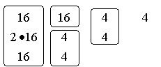
box-size we construct Table 1 - 3. Table 1 shows the behaviour when
increasing the box-size in the fractal on level n = 2 Fig. 18 where the first column represent the 64 filled boxes, 16 with one l2-particle, 16 boxes with a quarter
of a lL-particle, 16 boxes with a quarter of a Ll-particle and 16 where a L2-particle cover 16 boxes. The next
column represent the next box-size where each part of the lL particles lies in
the same boxes as the l2-particles and all parts of the four Ll particles moves into
the same box and the L2 particle now cover four boxes. We then have 16 boxes containing ![]() four boxes containing
Ll
and four boxes of
four boxes containing
Ll
and four boxes of ![]() . At the next level we have 4 boxes of
. At the next level we have 4 boxes of ![]() and four with
and four with ![]() . In the last level we have four boxes containing
. In the last level we have four boxes containing ![]() .
.
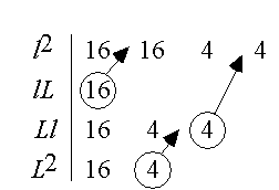
Table 1. This is the behaviour when
decreasing the box size on the level n = 2
snowflake fractal, Fig. 18. The columns show the contents in the
"filled" boxes of sizes (1/16), (1/8),
(1/4) and (1/2)
respectively.
Table
2 and 3 show the same decrease of the box size for the snowflake fractal
at level n = 3 and n = 4 respectively.
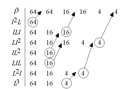
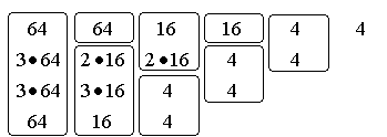
Table 2. This is the behaviour when
decreasing the box size on the level n = 3
fractal,. The columns shows the contents in the "filled" boxes of
sizes (1/64), (1/32), (1/16), (1/8),
(1/4) and (1/2)
respectively.
We can see from Table 1 - 3 that the number of boxes containing the same set of
particles can be written as ![]() see Table 4. A study of the contents in the
boxes shows that the coefficient
see Table 4. A study of the contents in the
boxes shows that the coefficient ![]() are given by
are given by
![]() (72)
(72)
where we can find recursive rules for ![]() and
and ![]() , see the result in the appendix of Paper II.
, see the result in the appendix of Paper II.
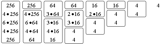
Table
3. This is the behaviour when decreasing the box size on the level n = 4 fractal. The columns show the contents in the
"filled" boxes of sizes (1/256),
(1/128), (1/64), (1/32), (1/16), (1/8), (1/4) and (1/2)
respectively.
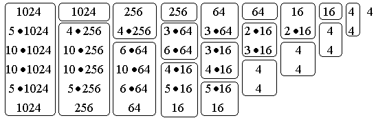
Table
4. This shows the coefficients for the fractal at level n = 2, 3, 4 and 5 with
the possible box levels m. The
coefficients inside the boxes are coefficients with the same probability
(measure).
If we bring the probabilities and the coefficients into the same table, Table 5
we see that we can find a similar recursive expression for the probabilities.
The complete solution to the box-counting problem is presented in the appendix
of paper II.
level n = 2
Coefficients:
4
4 4
16 4 4
16 32 16
Probabilities:
4
8 8
32 16 16
64 64 64
___________________________________________
level n = 3
Coefficients:
4
4 4
16 4 4
16 32 4 4
64 32 48 16
64 192 192 64
Probabilities:
4
8 8
32 16 16
64 64 32 32
256 128 128 128
512 512 512 512
___________________________________________
level n = 4
Coefficients:
4
4 4
16 4 4
16 32 4 4
64 32 48 4 4
64 192 48 64 16
256 192 384 256 64
256 1024 1536 1024 256
Probabilities:
4
8 8
32 16 16
64 64 32 32
256 128 128 64 64
512 512 256 256 256
2048 1024 1024 1024 1024
4096 4096 4096 4096 4096
Table
5. This shows the coefficients and the probabilities for the fractal at level n = 2, 3, and 4. This
table is used to find recursive relation for the probabilities of the snowflake
fractal.
The box-counting solution to the snowflake multifractal consist of two families. This is due to the box-sizes compared with the
contents in the boxes. We call the different families, the odd and the even.
The first box-size is odd and has the same size as the smallest particles. Next
box-size is even, next odd, and so on. Each corner of the odd box-sizes consist
of a boxes containing reduced copies of the whole fractal. This gives, for
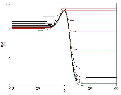
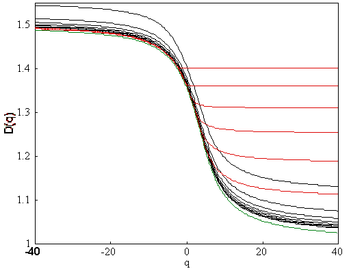
large negative q-values an exact value of a and therefore D-∞. In Fig. 21 - Fig. 28 the black curves are
solution with box-sizes larger than the largest particle, that in the middle.
The red curves are solutions with box-sizes smaller than the largest particle.
The convergence of the solutions is discussed in detail in paper II. All
solutions below are calculated from the fractal at level n = 90, i.e., the
number of particles in the fractal is 490 ≈ 1.53·1054. The curves in the
even family are for box-levels m = 10, 20, ..., 160 and the odd families for levels m = 9, 19, ..., 159.
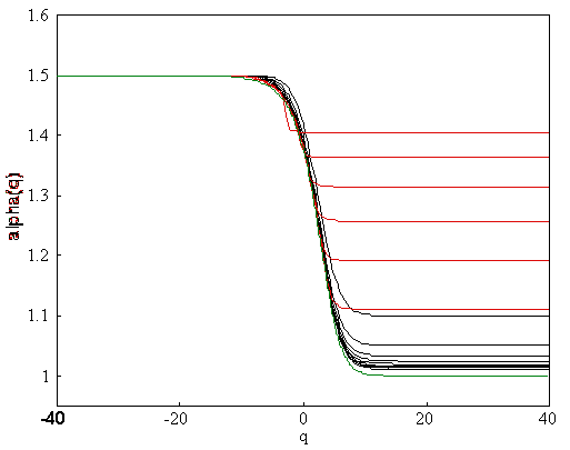
Figure
21. This is the function a(q) for the odd family. The black curves are
solutions for boxes larger than the largest particle, the red curves are
solutions for boxes smaller than the largest particle and the green is the
exact solution.
This sets of solutions are compared with the exact solutions, the green curves,
calculated from the analytical expressions Eq. (73) - (75) from paper I and II.
 (73)
(73)
![]() (74)
(74)
and
 (75)
(75)
Figure
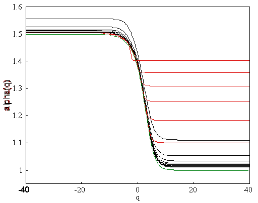
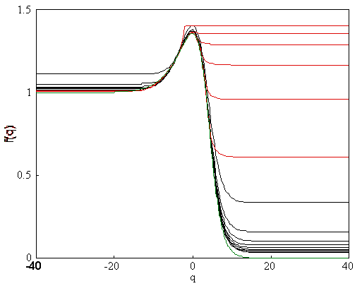
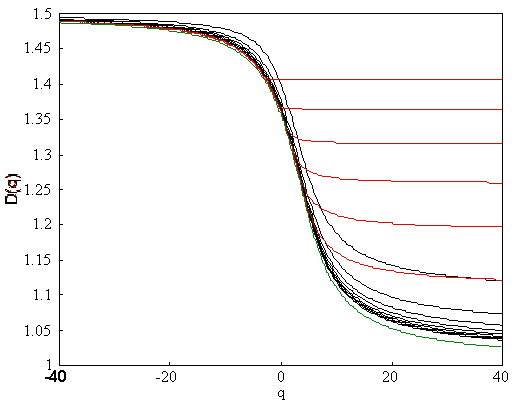
22. This is the function a(q) for the even family. The black curves are
solutions for boxes larger than the largest particle, the red curves are
solutions for boxes smaller than the largest particle and the green is the
exact solution.
In Fig. 21 and 22 we show the function a(q) for the odd and the even family respectively.
As we can see, smaller box-sizes give the best result for negative q-values and large
box-sizes give solutions which converge fast for positive q:s.
Figure 23 and 24 shows the function f(q) for the odd and the even family respectively.
As for a(q), the smaller box-sizes give the best result for
negative q-values
and large box-sizes give solutions which converge fast for positive q:s
Figure
23. This is the function f(q) for
the even family. The black curves are solutions for boxes larger than the
largest particle, the red curves are solutions for boxes smaller than the
largest particle and the green is the exact solution.
Figure
24. This is the function f(q) for
the even family. The black curves are solutions for boxes larger than the
largest particle, the red curves are solutions for boxes smaller than the
largest particle and the green is the exact solution.
If we plot f(q) versus a(q) we get the f(a)-spectrum, Fig. 25 and Fig. 26. Figure 25 show the odd family and Figure 26 the
even family. Compare these figures with those in paper II. The solutions in
paper II are calculated from the fractal level n = 16, i.e., 416 ≈ 4.3·109 particles and the
solutions below from level n = 90.
We observe that the red curves, i.e., solutions
for box-sizes smaller than the largest particles are closer to the exact
solution at the right side of the f(a)-spectrum. This side correspond to negative
values of the momentum q. The left part of the f(a)-spectrum, i.e., for
positive q-values,
boxes of sizes larger than the largest particle, that in the middle of the
snowflake, lies closer to the exact solution, the green curve.
This observation is important in the
calculation of the f(a)-spectrum. To get a good result in such a calculation it is important to vary the
sizes of the boxes and then select the left-most value of a for each f both on the right-
and the left part of the f(a)-spectrum.
We also observe that for the odd family all
curves ends up at the exact value of a , i.e., a = 1.5. The f(a)-spectrum start at the
point (1, 0) and ends up in the point (1.5, 1). We can understand this since the first point
correspond to the limit where q ® ∞. This limit is dominated by the largest particles in the fractal, since
that part gives the largest probability see Eq. (17). Since we only have one
particle with the largest size the value of f ® 0. The value of a is also given since the largest particle
consist of 4n particles of size 4-n at each level, and a ® ln(4n)/ln(1/4-n) = 1.
Figure
25. This is the f(a)-spectrum
for the even family. The black curves are solutions for boxes larger than the
largest particle, the red curves are solutions for boxes smaller than the
largest particle and the green is the exact solution.
Similarly we can understand the values at the
end point of the f(a)-spectrum since this is dominates by the
smallest particles when
q ®
-∞. At this point we
have 4n particles of size 4-n , i.e., f ® ln(4n)/ln(1/4-n) = 1 and the fractal
consists of 8n particles of size 4-n hence a ® ln(8n)/ln(1/4-n) = ln(8)/ln(4) = 1.5.
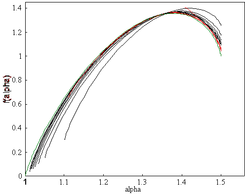
Figure
26. This is the f(a)-spectrum
for the odd family. The black curves are solutions for boxes larger than the
largest particle, the red curves are solutions for boxes smaller than the
largest particle and the green is the exact solution.
In Fig. 27 and Fig. 28 we show the generalized
dimensions Dq(q) for the even and odd family respectively. As
we can see, smaller boxes is best for negative values of q and larger boxes for
positive q:s.
By varying the box-size and select the smallest value of Dq for each value of q, we can extract the
closest solution to the exact curve.
Figure
27. This is the Generalized dimension Dq for
the even family. The black curves are solutions for boxes larger than the
largest particle, the red curves are solutions for boxes smaller than the
largest particle and the green is the exact solution.
We also observe that the odd family converge
fastest, special for negative values of the momentum q. This is due to the
fact that this family have a large number of boxes containing reduced copies of
the whole snowflake fractal.
Figure
28. This is the Generalized dimension Dq for
the odd family. The black curves are solutions for boxes larger than the
largest particle, the red curves are solutions for boxes smaller than the
largest particle and the green is the exact solution.
3.7:
Box-counting on a gas evaporated metal particle aggregate
One goal in the calculations of fractal dimensions of aggregates, is to
compare with the dimensions given by different computer aggregation models.
Such models have been proven to be useful, in order to understand the processes
that give rise to fractal structures.
3.7.1: Diffusion Limited Aggregations
One common computer model is DLA, Diffusion Limited Aggregation. This model has been found to be relevant to a large variety of
processes including fluid-fluid displacement in porous media, dielectric
breakdown, electrode position and possibly growth processes. The DLA model illustrates that simple growth
and aggregation models could lead to valuable insights into important physical
and chemical processes.
Figure
29. The DLA model in two dimensions. Start with a single occupied site (the
centre). Place a single particle at a random position on a circle outside the
cluster and use random walk on a lattice. If the particle hits the cluster it
grows with the lattice size, if it walks outside the outer circle, take a new
particle on the starting circle.
In a DLA model we place a particle from a randomly selected point on a circle
outside the cluster. This particle can move on a lattice with random walk. If the particle hits the cluster it stops and the cluster grows with one cell. On the other hand, if the
particle moves outside an outer circle, we place a new particle at a randomly
selected point on the starting circle. The simulation starts with a single
occupied site, the black one in the middle.
This simple two-dimensional model can be
modified (generalized) in different ways. A common generalisation is to
introduce a sticking probability S ≤ 1. The Hausdorff dimension given by the DLA model in two
dimensions is D0 = 1.70 ± 0.06 for S = 1 and D0 = 1.72 ± 0.06 for S = 0.25 [20].
3.7.2: Ballistic Aggregations
This model was one of the first cluster
aggregations models, developed by M. J. Vold, more than 25 years ago [20]. In
contrast to DLA, with a small mean free path compared with the size of the
aggregate, the mean free path of the ballistic models is large. We begin with a
single stationary particle, and one free particle in a random ballistic
(linear) trajectory in the vicinity of the stationary particle. If the
ballistic particle hits the stationary it sticks to that point and a stationary
cluster is formed. Then we add new ballistic particles, one at a time, until a
large cluster has formed.
A ballistic aggregate becomes very dense and
the fractal dimension is very close to the Euclidean dimension of the embedding
space. For large clusters, up to 250 000 particles, the Hausdorff dimension is
larger than 1.95 in two, and larger
than 2.3 in three dimensional simulations[20].
3.7.3: Cluster-Cluster Aggregations
In this models we consider a squared lattice, L by L with L2 sites. We place N particles at random positions
on the lattice and let them move randomly. On collisions they stick, and form
larger and larger clusters that can collide with other cluster. In the final
state we have one large cluster. There are many extensions to cluster-cluster
aggregations, the cluster can rotate and the lattice can be multidimensional
etc. Three common versions of cluster-cluster aggregation is DLCA,
Diffusion-Limited Cluster-Cluster Aggregation where the cluster moves with
random walk, Ballistic cluster-cluster aggregation where each cluster moves
along ballistic (linear) trajectories and the chemical cluster-cluster
aggregation. The last model is the same as the ballistic but with vanishing
sticking probability. In this limit, the clusters have time to investigate all
the possible sticking situations before choosing one. This model is used to
study colloids, where we have a strong repulsive barrier that the particles
must overcome before being attracted by the short range Van der Waals forces.
The theoretical results of cluster-cluster dimensionis 1.44 and 1.78 in a two
and three dimensional simulation respectively. If ballistic trajectories are
used the dimensions are 1.55 and 1.91 and in a cluster-cluster chemical
simulation the result is 1.55 and 2.04 [20].
3.7.4: Aggregate of magnetic particles
In paper III we study a fractal aggregate of magnetic cobalt particles. The
aggregate were produced by inert-gas evaporation[21] from a heated tungsten
spiral in a conventional bell-jar system. The evaporation took place in 1.3 kPa
of argon gas and resulted in particles of about 100 Å radius that were
clustered into large connected aggregate as seen in Fig. 30. Particles interacting via long-range forces
produce aggregate with quite different scaling properties [22]. We estimated
the Hausdorff dimension of the fractal to be 1.703 ± 0.006.
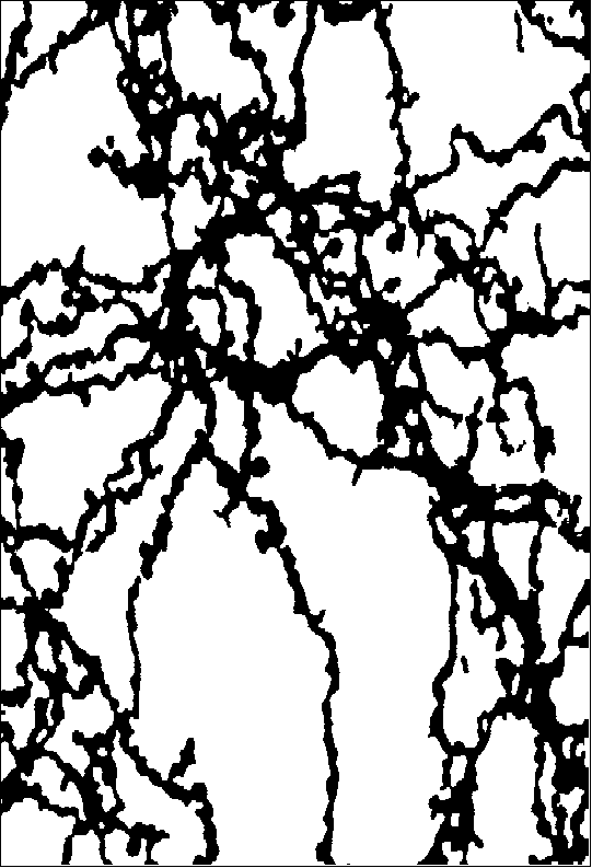
Figure
30. A fractal aggregate of gas-evaporated magnetic cobalt particles..
REFERENCES:
[1] W. F. Ganong, Review of Medical Physiology, Sth Ed. Lange
Medical
Publications, California
1977.
[2] Peitgen, H. O., and Richter, Peter, The Beauty of Fractals
(1986).
[3] B. B. Mandelbrot, Les Object Fractals, Flammarion, Paris 1975.
- B. B.
Mandelbrot, Fractals:
Form, Chance and Dimensions, Freeman, San
Fransisco 1977. B. B.
Mandelbrot The Fractal Geometry of
Nature,
Freeman, San Fransisco 1982.
[4] F. Hausdorff, Dimension und äußeres Maß, Mathematische Annalen 79,
157 (1919).
[5] Fleischmann, M., and Teldesley, D.J., eds., Fractals in the Natural
Sciences
(1990);
[6] Hideki, Takayasu, Fractals in the Physical Sciences (1990);
[7] Gleick, James, Chaos: Making a New Science
(1987);
[8] J.-P. Eckmenn and D. Ruelle, "Ergodic Theory of Chaos and
Strange
Attractors," Rev. Mod.
Phys. 57, 617 (1985)
[9] J. Guckenheimer and P. Holmes, "Nonlinear Oscillations,
Dynamical
Systems, and Bifurcations of
Vector Fields", Appl. Math. Sci. 42, Springer,
New York (1983).
[10] K. J. Falconer, The
Geometry of Fractal Sets. Cambridg
University Press.
Cambridge 1985.
[11] L. Pietronero and E. Tosatti (eds.), Fractals in Physics.
North-Holland,
Amsterdam 1986.
[12] J. Feder, Fractals, Plenum Press, New York 1988.
[13] T. C. Halsey, M. H. Jensen, L. P. Kadanoff, I. Procaccia and B. I.
Shraiman, Phys. Rev. A 33,
1141 (1986).
[14] H. G. E. Hentschel and I. Procaccia, Physica D 8, 435 (1983).
[15] B. B. Mandelbrot, J. Fluid. Mech. 62, 331 (1974).
[16] P. Grassberger, Phys. Lett. 97 A, 227 (1983); 107 A, 101 (1985).
[17] A. Renyi, Probability Theory, North Holland, Amsterdam (1970)
[18] C. Amitrano, A. Coniglio, F. dj Liberto, Phys. Rev. Lett. 57 1016
(1986). -
Y. Hayakawa, S. Sato, M. Matsushita,
Phys. Rev. A 36 1963 (1987).
[19] J. D. Farmer, Z. Naturforsch. 37 a, 1304 (1982).
[20] P. Meakin, Computer Simulations of growth and aggregation processes
in On Growth and Form
(edited by H. E. Stanley and N. Ostrowsky)
1986, Martinus Nijhoff
Publishers, Dordrecht.
[21] C. G. Granqvist, R. A. Buhrman. J. Appl. Phys. 47, 2200 (1976)
[22] G. Helsen, A. T. Skjeltorm, P. M. Mors, R. Boet and R. Jullien,
Phys. Rev.
Lett. 61, 1736 (1988).